Seismic Probabilities for Reservoir Simulation
Seismic reservoir characterization is usually based on the interpretation of seismic attributes that relate to the geological feature or reservoir property of interest. If we are interested in fault geometries, there is a variety of geometric attributes that we can use to map the details of fault distributions and constrain discontinuities and flow barriers in geological and flow simulation models. If we are interested in reservoir properties, however, the usual approach is to estimate seismic attributes that are qualitatively related to such properties. The interpretation of the attribute focuses on the identification of “good” and “bad” areas depending on how the attribute relates to the property of interest.
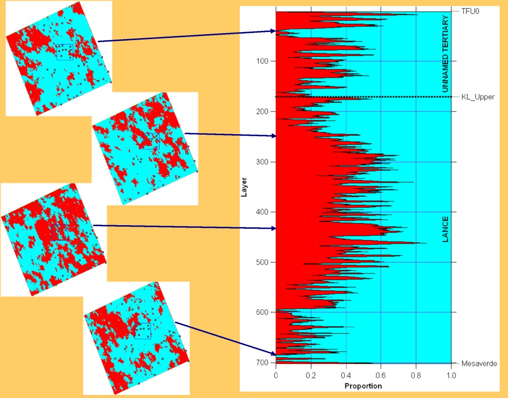
Figure 1 : Examples of facies maps extracted from layers of 3D facies model built using log and seismic data. By definition, proportions of channel (red) and non channel (cyan) facies in the maps are consistent with proportions indicated by the vertical proportion curves for the corresponding layer.
Often we must go beyond qualitative interpretations and build a geological model that can be later transformed into a flow simulation model. Therefore we must do more than simply separate good and bad areas. A flow simulation model often requires much more than a simple porosity field generated by applying a linear regression between impedance and porosity.
While simple models may be all we need to simulate fluid flow in certain geological settings, complex geological or fluid variations may require additional information before meaningful fluid flow simulation is attempted. Fluvial sandstone reservoirs of low porosity and low permeability are a good example of reservoirs that require complex geological models to properly describe their internal architecture. These reservoirs are typically referred to in the literature as “tight”. Geological facies are the key parameter when performing geomodeling and simulation of these reservoirs.
We apply a statistical workflow to classify and map facies based on log and seismic data. Facies are then used as the basis to distribute porosity and permeability across the reservoir. Our approach combines geologic determinism to analyze log data with statistical approaches to analyze seismic data and indicator-based geostatistics to model single and multi-story channel facies with appropriate spatial and geometric statistics. Unlike commonly used approaches to map facies or lithologies from seismic data based on coloring “independent” regions in seismic attribute crossplots, our approach accounts properly for overlap among different scenarios and quantifies the probability of their occurrence.
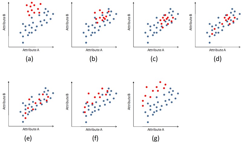
Figure 2 : Conceptual crossplots of two seismic attributes colorcoded by another variable related to the reservoir property of interest. The target (gas saturated sandstones, for instance) is colored in red and the background is colored in blue. (a) Good separation between background and clustered target. (b) Partial separation, clustered target. (c) No separation, clustered target. (d) No separation, partially clustered target. (e) No separation, unclustered target. (f) Partial separation, unclustered target. (g) Good separation, unclustered target. Using our statistical approach, it is possible to assign probabilities to the target even when it does not separate well from the background (cases b, c, d, and f) where the response is at least clustered or partially clustered around a certain region. This approach won't yield reliable results in case (e) when the background and the target cover the same area in the crossplot. In this case the probability of the target will be the same for all attribute values.
Seismic Probabilities for Simulation Workflow
- Petrophysics: The result of this step is a normalized set of enhanced logs that are used for seismic-well calibration, stratigraphic interpretation, and facies classification.
- Log scale lithology and facies classification: Facies associations are developed based upon the dominant lithology and thickness of each interval.
- Crossplot of impedances at log scale: Rock physics analysis of well log data indicates that seismic attributes derived from 3D pre-stack seismic data may be good indicators of the presence of sands.
- Stratigraphy: Several iterations are required to ensure consistency between seismic horizons and well markers.
- Vertical facies proportion curves: The intervals of interest are divided into a fixed number of layers. The total thickness of each facies for all wells is calculated for each layer and the relative proportions of the different facies by layer are computed.
- Crossplot of impedances at seismic scales: Acoustic and shear impedance volumes are converted to depth. Seismic-scale acoustic and shear impedances are extracted at each well location and colored by log scale lithology and facies flags.
- Facies probabilities from seismic: 3D probabilities of channels based on acoustic vs shear impedance crossplots are computed using the “Probabilities from crossplots” approach.
- 3D facies modeling: The facies probabilities estimated from seismic impedances in depth are mapped onto the stratigraphic grid and rescaled layer by layer to match the global vertical proportion curves. This result is used as secondary data to constrain the lateral distribution of facies using sequential indicator simulation.
- Porosity and permeability distribution: Porosity is distributed on the seismic-constrained facies models using facies-dependent variograms and sequential Gaussian simulation while also honoring log data and porosity statistics per facies.
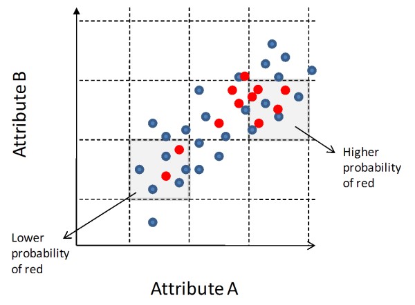
“Probabilities from crossplots” approach: We use conditional probabilities and the correspondence of the different log scale scenarios with seismic scale attributes sampled at well locations to estimate the likelihood of the desired scenario away from wells.
|
Figure 3 : Probability estimations from crossplots. A rectangular grid is superimposed on the crossplot and individual probabilities of the different scenarios (red and blue in this example) are calculated for each rectangle. These probabilities are then assigned to the whole seismic volume. |
Our workflow estimates facies probabilities from log and seismic data and we use this information to constrain the facies distribution in the reservoir. Our workflow starts by performing careful petrophysical and geological analysis which results in a set of facies logs that are used to help the characterization of facies at three different scales. Local facies curves and vertical proportion curves are treated as hard data whereas seismic derived probabilities are used as soft constraints when building the geomodel and distributing facies using sequential indicator simulation. Facies are the key parameter when modeling tight gas sand reservoirs as they can control which areas of the reservoir are more prolific.
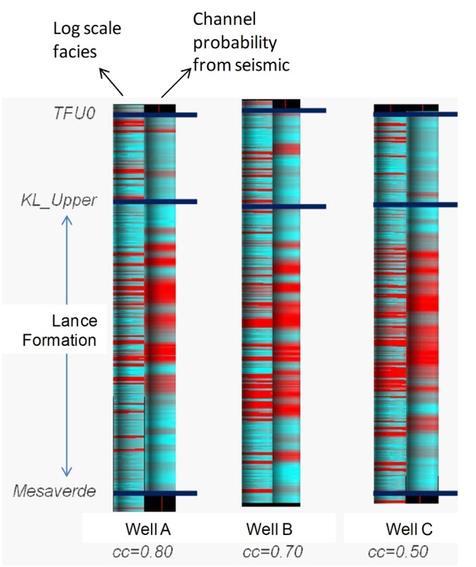
Figure 4 : Comparison of log scale facies with channel probabilities estimated from seismic data for 3 different wells. Log scale facies (left figure at each well location) vary from 1 (shaly floodplains, cyan) to 4 (multistory channels, red). Channel probabilities from seismic (right figure at each well location) vary from low (cyan) to high (red). Notice how channel probabilities correlate well with thicker stacks of channels, even though these channel probabilities are not able to separate individual multistory channels observed at well locations.
For more information: “Constraining 3D facies modeling by seismic derived facies probabilities: example from Jonah Field tight gas”, Reinaldo J. Michelena, Kevin S. Godbey and Omar Angola, The Leading Edge 2009, in press.